Motivation
The master’s course “Building and Mining Knowledge Graphs” required us to work on an individual project. I decided to challenge myself with accessing and converting the MusicBrainz dataset into a knowledge graph before linking it to a few metrics for each country existing in it. Thereby deploying the MusicBrainz’ postgreSQL database using docker, and focussing on the research of conversion by using three different approaches. The linking part on the other hand turned out to be too easy, hence I plan to connect the MusicBrainz dataset to my Spotify listening history in a follow-up project.
The code is on github: https://github.com/arthurhaas/um_project_knowledge_graph
Steps
The below figure illustrates my process of gathering the three datasets, converting them into triples a.k.a. creating a knowledge graph, linking all three, and storing them inside GraphDB for querying with SPARQL.
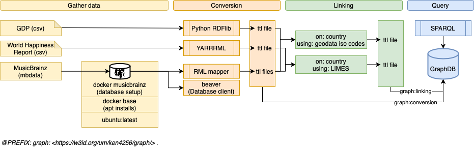
Technical setup of the project from data ingest to querying GraphDB.
/1 Gather data
As you see in the above illustration, I used three datasets. All of these datasets contain the country as a common entity, which will be used for linking later.
- MusicBrainz is a large collection of music data about artists, their albums, songs, etc.
- The Happiness Report indicates the population’s happiness.
- The report of the GDP per capita shows the economic status of a country.
Downloading the three datasets and making them usable was the first step of the project. While the Happiness Report and GDP Data were combined around 0.5 MB, the size of the MusicBrainz dataset totals roughly 50 GBs. Hence, I had to make a choice about which part of the MusicBrainz data to use. I decided to use the core data for the knowledge graph. Furthermore, to make the MusicBrainz dataset usable, a setup concerning docker, postgreSQL, and mbdata was required. MusicBrainz recommends using mbdata instead of their own MusicBrainz Server System, in case the webserver is not required. Since I only need the dataset, mbdata was sufficient. To achieve this, I’ve set up an ubuntu docker base image and followed the tutorial on mbdata’s GitHub repository. This was not complete in terms of which commands to execute, hence I had to do a great amount of engineering research to make the database runnable. Details won’t be mentioned here but can be found in the corresponding Dockerfiles and readmes.
/2 Conversion
Before starting to convert the datasets, it is wise to conceptionalize the final knowledge graph. Next figure shows that.
Concept of the knowledge graph to build to plan entity IRIs, relations and literals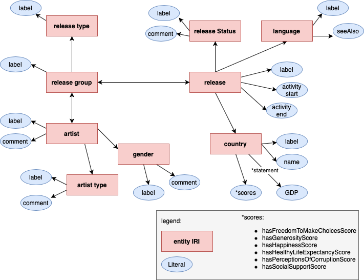
Conversion method 1: YARRRML
For converting the happiness report csv file into the turtle syntax YARRRML was used, which is a YAML syntax for RML rules.
| |
Conversion method 2: Python with rdflib
For converting the GDP data, I have decided to experiment with a python library called rdflib. Using this was very flexible due to the programming language python. To convert the dataset, pandas was used to store the csv file and iterate it line by line. The tricky part was the binding of a namespace to make it appear as a correctly written prefix in turtle syntax.
Source table:
| Country Name | Country Code | Indicator Name | … | 2019 |
|---|---|---|---|---|
| Germany | DEU | GDP per capita (current US$) | … | 46445.2491012508 |
Python code:
| |
Resulting turtle syntax:
| |
Conversion method 3: plain RML on postgreSQL database
The most challenging dataset was MusicBrainz due to its complexity with over 200 tables. I have decided to use plain RML. To create a working connection to a postgreSQL server I had to look into RML test cases because the documentation is too sparse. In addition, I decided to split the RML mapping into files corresponding to entities like country, releases, release groups, and artists to avoid one large monolith job.
A small extract from mapping the artists from postgreSQL to turtle using a query:
| |
/3 Linking
For the link between GDP and MusicBrianz a mapping file from geonames was used because the link was made between and iso-2 and an iso-3 country code, straightforward. For the link between the happiness report and MusicBrainz on the other hand, LIMES was applied.
/4 Query using SPARQL on GraphDB
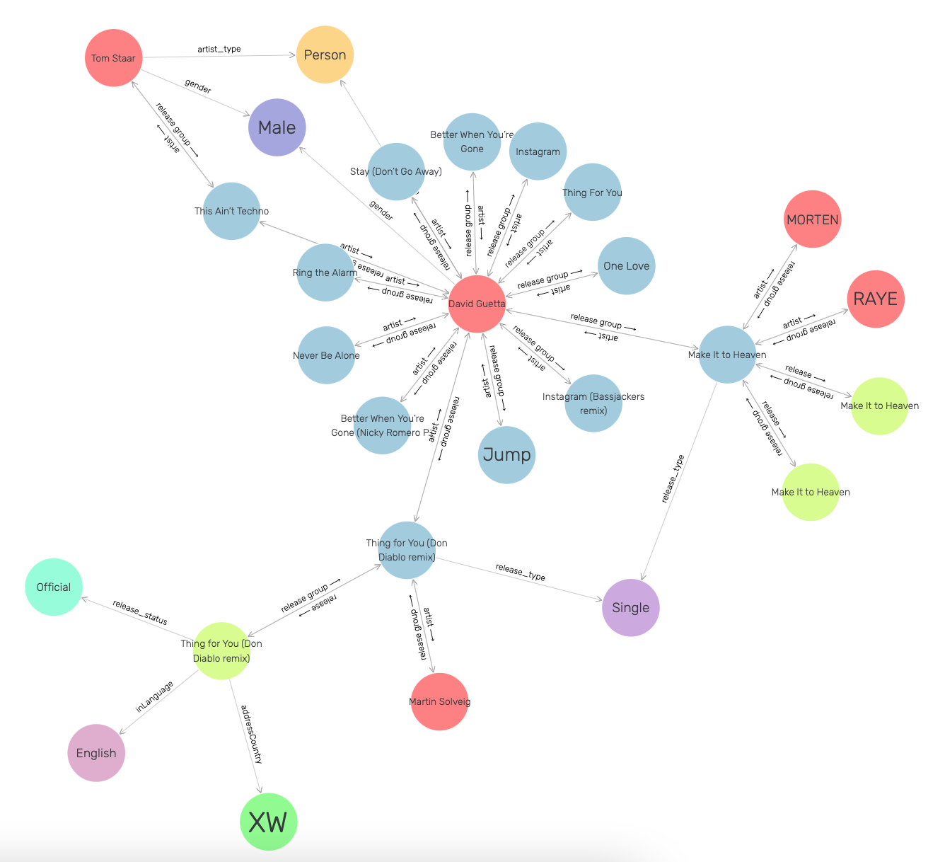
After conversion and linking, the data was loaded into GraphDB. The title illustration shows an overview of some entities and relations as they are displayed in GraphDB’s web app.
As an example, the following SPARQL query returns the total number of releases by country in descending order.
| |
Next up
Expanding the linking step from simple metrics by country to my Spotify listening history is the next step of this side-project. I collect my listening history by “scrobbling” to https://www.last.fm.
Further Spotify API’s I am interested in trying out: